-
Overview of Exporting to Excel
If your Estimate Grid has a large amount of estimates or you wish to perform analysis or metrics for the Estimate Grid, you can export the entire grid to Excel. Once exported, you can analyse, perform metrics and create visualisations of your data.

-
Click on the Export to Excel button
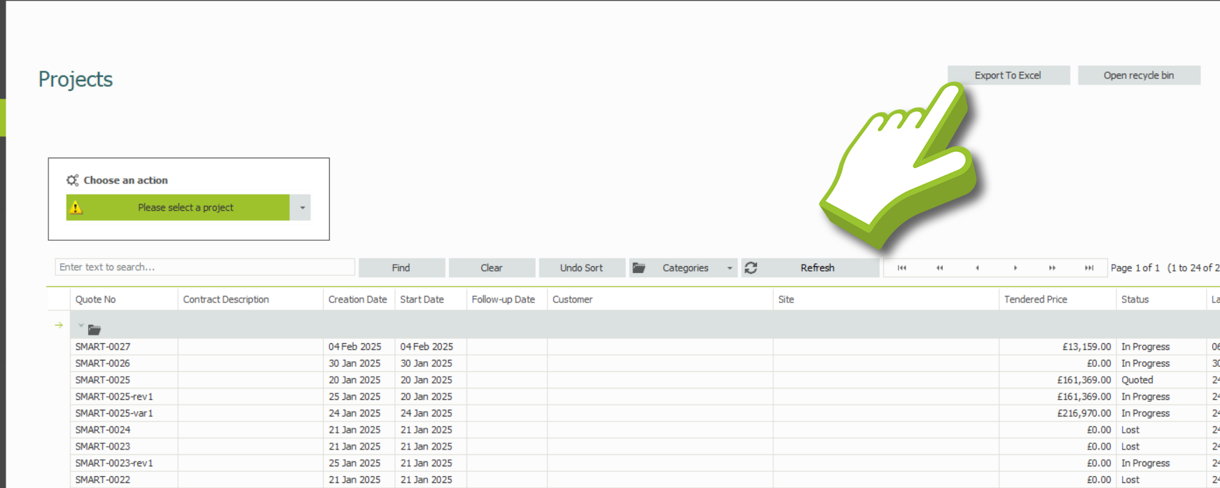
From the Home screen, navigate to the Projects tab to access the Hub. At the top right of the screen, you’ll see a button labeled Export To Excel. If you do not see it then either adjust the border width-wise till you find it or full-screen the application. Click on it and you’ll be taken to a File Explorer.

-
Save the Project List
Navigate to the location where you want to save your project list. Rename the file to your preferred name and press the Save button. The project list will be saved in .CSV grid format. This file can be opened in most spreadsheet programs, such as Microsoft Excel. If Excel is already installed on your computer, the .CSV file will typically open automatically.
-
Viewing and Formatting the Project List
Once the project list opens, you may notice that parts of the list have been clipped. This happens because the .CSV format only saves raw data without formatting.
To adjust the column widths and view all the content clearly (in this example using Microsoft Excel): Click the Format Tool, then select Autofit Column Width to resize all columns and display the entire project list.
-
Creating a Table from the Estimate Grid
Now that we’ve formatted the data, your Estimate Grid is ready for analysis and metrics. We can filter the data further by creating a table from the Estimate. Begin by selecting all of the data of your Estimate Grid and then navigate to the Insert tab, then click on the Table button. A new table toolbar will appear with your data formatted in default styling.

Now that it’s a table in Excel, you can customise the look of your table by adding Banded Rows or Banded Columns. You can also use the Table Styles option to modify the Table colours.

Now we can use the Filter Buttons on the right of the Header Row on each cell to organise the data on the Table. This can be done by Sorting them adding Text Filters or by Filtering the Data.
Sorting Options
On the top of the filter window, when you click on the Filter button. You can sort the data from A to Z, Newest to Oldest and Smallest to Largest and vice versa.
Filtering the Data
Once you click on the Filter button at the bottom of the filter window, you can filter what is shown in the table. You can do this by selecting or deselecting the options below.
Inserting a Slicer
Finally, you can insert a slicer if you would like to quickly filter the criteria on the table. Click on the Insert Slicer button, select what you wish to filter and a Slicer will be placed on the Excel canvas.
SMART Estimator
What’s new?
Getting Started
Setup and Configuration
-
Enterprise Server
-
Cloud Server Setup
Local Windows Server Setup
Adding Cloud server users
Server Back Up and Restore
Archiving Estimates from server
Migrating Local server to Cloud
Creating Folders in Enterprise Server
Using Server Tools from the Command Line
-
User software settings
User Address Settings and Yard
Scaffold Banner and Sheeting logo
Adding Watermarks
-
Setting up your Rates
Editing Shared Pricing Rates
Creating a rate setting template project
Importing and Exporting shared Rates
Creating an Estimate
Importing Drawings and Models
Scheduling Scaffolds
Creating 3D Scaffolds
-
3D Model Controls
Adding Independent scaffolds
Adding Circular Tank scaffolds
Adding Birdcage & Lift shaft scaffolds
Adding Tied or Freestanding towers
Adding Stair towers, Ladders towers & Buttresses
Adding Loading bays
Adding Chimney scaffolds
Adding Temporary Roof
Adding Edge protection
Adding Pavement Gantry’s
System Scaffolds
Safety Decking
Using the Scaffold Library
Editing Scaffolds
Scaffold Add-ons & Options
-
Adding Gin wheels, Rubbish Chutes, Safety standards, Double standards and Lamps
Adding and Editing bridges/beam work
Adding Beams around Corners
Adding Cladding
Adding Cantilever protection fans
Adding Pavement Lifts
Adding Recesses and Infills
Building and Ground colour
Visual options (Tube, Ladder, System details and Grips)
Add a Pedestrian or Scaffolder
Copying pictures of the model
Material Lists and Drawings
Pricing and Estimation
Quotations
Enterprise Server
Troubleshooting